Blog

In our last blog post, we introduced neural sparse search, a new efficient method of semantic retrieval made generally available in OpenSearch 2.11. We released two sparse encoding models on OpenSearch model hub and Hugging Face model hub. Both models excel at producing relevant information compared to other sparse encoding models with the same architecture. Sparse search uses a Lucene inverted index to achieve high-quality semantic search with low resource overhead.

In this blog post, we first explain the basics of neural sparse search and quantify its efficiency. We then explore two methods of speeding up neural sparse search: a Lucene upgrade and GPU acceleration. With a Lucene upgrade, the P99 search latency for the doc-only and bi-encoder modes is reduced by 72% and 76%, respectively. With a GPU endpoint, the P99 search latency for the bi-encoder mode is reduced by 73%, and the neural sparse ingestion throughput is increased by 234%.

For key takeaways, see the Conclusions section.

BM25 search

Before diving into neural sparse search, let’s first take a brief look at how the traditional BM25 search works so that we can compare the two.

In OpenSearch, the basic search functionality is built on top of a Lucene inverted index. For each term in the index, the Lucene inverted index maintains a posting list. The posting list stores all documents containing the term, sorted by internal document ID. When you run a basic match query in OpenSearch, the query text is tokenized and transformed into Lucene disjunctive term queries, such as TermQuery(termA) OR TermQuery(termB) OR TermQuery(termC) .... Lucene then searches the posting lists for all query terms, as shown in the following image.

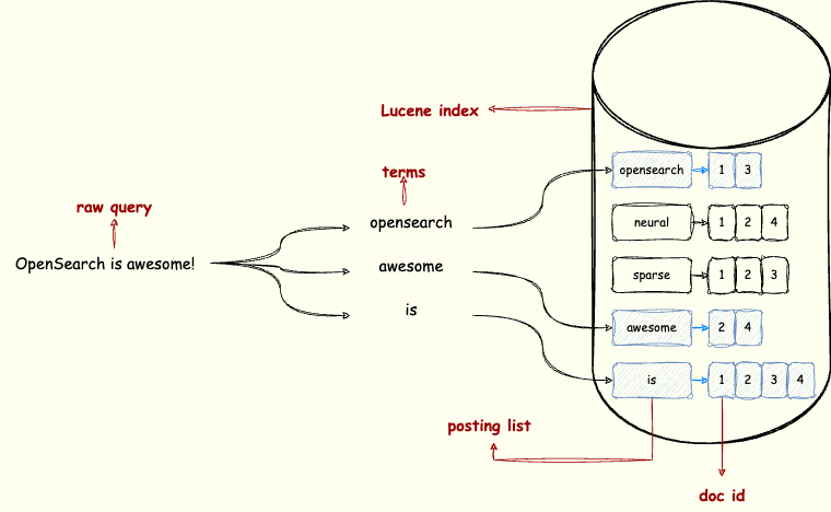
Lucene merges the selected posting lists and calculates document scores in real time using the BM25 algorithm. The overall time complexity is determined by the number of hit posting lists and the lists’ lengths. Although Lucene implements many optimizations, like block scoring, MaxScore, and WAND, this is how the search works at a high level.

Neural sparse search basics

For neural sparse search, the fundamental workflow is very similar to BM25. Let’s compare neural sparse search to BM25 in terms of latency at ingestion time and query time.

Ingestion time

At ingestion time, neural sparse search processes text differently compared to BM25. The most significant difference is that neural sparse search uses neural models to transform the raw text into tokens and their corresponding weights. These token/weight pairs comprise a sparse vector. The neural model expands the tokens with synonyms and generates token weights based on their semantic importance. Next, similarly to BM25, Lucene creates a posting list for each token. The only difference in this process is how the fields are stored. Neural sparse search stores the fields in the Lucene FeatureField, while BM25 stores a standard OpenSearch text field in the Lucene Field. The difference in storage and its impact on search latency are negligible. As we discuss in the following sections, in most cases, the bottleneck for ingestion throughput is model inference.

Query time

At query time, the search process consists of two parts: building the sparse vector and searching the inverted index. Neural sparse search has two modes: doc-only and bi-encoder:

• For the doc-only mode, we use a tokenizer and a predefined lookup table to build the sparse vector. The tokenization takes less than 1 millisecond. In this mode, the query tokens are not expanded with synonyms, so all tokens must occur in the original query text.
• For the bi-encoder mode, we use a neural model to generate the sparse vector, just like we do during ingestion. Each query requires one model inference call. After we obtain the sparse vector, we transform it into Lucene disjunctive feature queries (FeatureQuery(termA) OR FeatureQuery(termB) OR FeatureQuery(termC) ...). Each FeatureQuery looks through the corresponding token’s posting list. Similarly to BM25, the search time complexity depends on the number of hit posting lists and the lists’ lengths. However, for neural sparse search, posting lists are longer (because of document expansion) and the bi-encoder needs to examine more posting lists (because of query expansion). Assuming all documents have a similar term frequency distribution, the length of posting lists grows proportionally to the number of documents. This means that the effort required to search the inverted index increases linearly with the number of documents in the dataset.

Accelerating inverted index search

To accelerate inverted index search, a common approach is horizontal scaling. OpenSearch distributes the documents in an index to multiple shards, each of which is a self-contained Lucene index. During the query phase, OpenSearch assigns a dedicated search thread to each shard. By adding more data nodes and distributing the shards evenly, we add more processing threads and distribute the search workload more efficiently. The workload for each thread decreases, leading to faster inverted index searches for both BM25 and neural sparse search.

Neural sparse search and BM25: Speed comparison

Having explored the inner workings of neural sparse search, a natural next step is to analyze its speed. Can we compare its performance quantitatively, especially against BM25?

Because the neural sparse search latency is proportional to the document count, this linear relationship can be expressed as (y = kx + b), where (y) is the client-side search latency and (x) is the document count. In this formula, (b) is the constant term of the linear function, which represents the latency that is not related to the inverted index (for example, network I/O, tokenization, or model inference). The constant (k) is the slope of the linear function. In this formula, it represents the time complexity of searching the inverted index. By sampling different document counts ((x)) and measuring the client-side latency ((y)), we can estimate (k) and (b) using the least squares approximation.

Benchmark tests

For benchmark tests, we used the following configuration:

• A cluster containing 3 r5.8xlarge data nodes and 1 r5.12xlarge leader/machine learning (ML) node
• OpenSearch version 2.12

To understand how document volume affects search speed, we performed experiments on the
MS MARCO dataset with document counts ranging from 1 million to 8 million, increasing by 1 million each time. To ensure consistent model inference times across these experiments, we set a fixed target throughput.

Benchmark results

The following figure shows the experiment results.

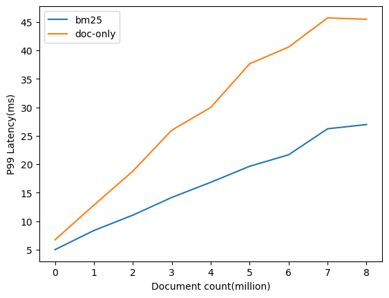
Note: For this blog post, we measured the client-side latency. The client-side latency consists of the sparse encoding model/sparse tokenizer inference time, retrieval time, and network latency.

The results shown in the preceding graph align with our theoretical expectations. Both search methods (BM25 and doc-only sparse search) show a linear increase in processing time as the number of documents increases. The approximate latency unrelated to the inverted index ((b)) is 5.4 ms for BM25 and 8.7 ms for doc-only sparse search. These numbers are very similar for BM25 and sparse search, indicating that the extra work required for tokenizer inference is very small. The approximate slope of the graphs, which represents the time complexity of searching the inverted index ((k)`) is 2.80 ms/1M docs for BM25 and 5.15 ms/1M docs for doc-only sparse search. Based on this, we can conclude that on the MS MARCO dataset, the retrieval latency for neural sparse doc-only mode is about 1.8x that of BM25. Thus, BM25 and doc-only sparse search latencies are comparable.

For the bi-encoder mode, the latency unrelated to the inverted index ((b)) is 265.4 ms, and the time complexity of searching the inverted index ((k)) is 20.58 ms/1M docs. The fixed term ((b)) is much larger than that of BM25 because of model inference. You can speed up model inference by using a GPU endpoint, as we show in Accelerating model inference using GPU. Additionally, because of query expansion, the retrieval latency for the bi-encoder mode is about 4x that of the doc-only mode.

Note that the exact slope value depends on the distribution of the data. This means that for different datasets, you may get different slopes. However, the relative difference between these slopes is likely to remain small. This is because the key factor influencing the slope is token expansion rate, which reflects the model’s ability to identify semantically related terms. This ability, ideally, should be consistent across datasets. The experiment results on the MS MARCO dataset serve as a strong reference point and can be used to estimate the latency of neural sparse search for other datasets.

For medium to large datasets (millions to tens of millions of documents), neural sparse search is very efficient, with smaller client-side latency and significantly lower resource consumption compared to dense vector search (see this blog post). The doc-only mode delivers a better client-side search latency, faster than the time required for ML inference. Neural sparse search provides additional cost savings because you don’t need to host a powerful ML service that supports a high throughput.

However, for extremely large datasets (billions of documents), the latency of neural sparse search also grows linearly with the number of documents. In this case, a dense vector search is a better choice for low latency because the latency of the underlying approximate nearest neighbor (ANN) algorithm used in dense vector search grows logarithmically with the number of documents. We’re actively working on improvements to neural sparse search to address its scalability limitations with extremely large datasets.

Accelerating sparse search with Lucene upgrades

In the past 20 years, Lucene has continually optimized its core performance, from streamlining index file I/O to improving posting list merging algorithms. Building neural sparse search on top of Lucene allowed us to take advantage of these optimizations. The optimizations are ongoing, and OpenSearch 2.12 uses the latest advancements in Lucene 9.9. Compared to Lucene 9.7, used in OpenSearch 2.11, Lucene 9.9 offers a significant performance boost, making it the fastest version yet (for more information, see the Lucene release notes). This improved performance extends to neural sparse search.

Because of its use of the top-k hits disjunctive Boolean query, neural sparse search performance improves with the new Lucene version. To demonstrate this, we conducted a performance comparison between OpenSearch 2.11 and 2.12 on the MS MARCO dataset. We used OpenSearch pretrained sparse encoding models on the same cluster setup mentioned previously, with each index having 3 primary shards and 1 replica shard. All indexes were force merged before the search in order to ensure consistency.

Benchmark results for 1M documents

The following figure shows the experiment results for 1M documents.

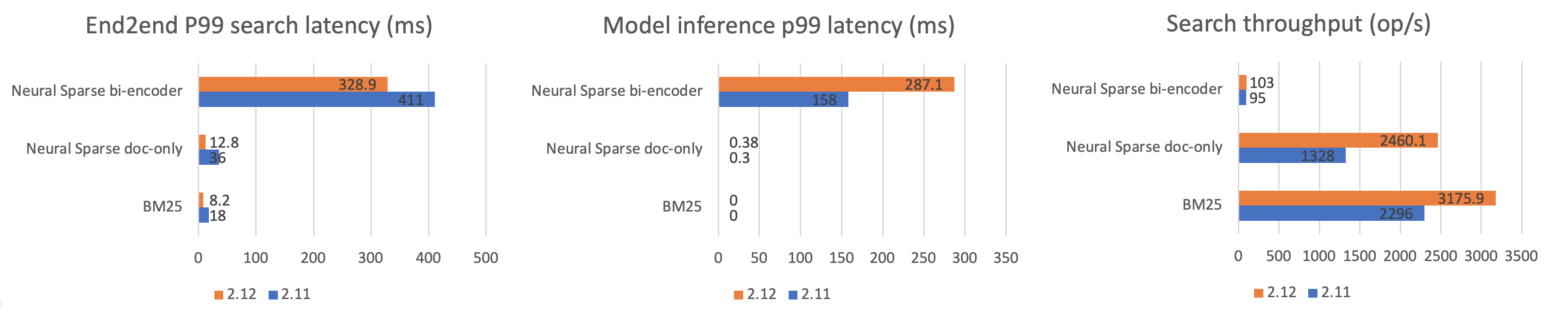
Benchmark results for 8.8M documents

The following figure shows the experiment results for 8.8M documents.

Results explained

The key takeaways from the experiment are:

1. For 8.8M documents, search speeds improve significantly for all search methods. The 8.8M dataset shows significant performance gains from Lucene optimizations. As mentioned previously, query latency includes the time needed for model inference and searching the inverted index. As the number of documents in an index increases, the time needed to search the inverted index grows linearly and becomes the dominant factor in the response time compared to model inference. For the bi-encoder mode, although the model inference time increases due to higher throughput, its overall latency still shows a significant reduction.
2. For 8.8M documents, neural sparse search benefits from Lucene optimizations more than BM25 does. This is because Lucene pruning algorithms like WAND and MAXScore struggle to efficiently handle the learned sparse weights used by neural search, compared to the term frequencies that BM25 relies on. Additionally, neural sparse search needs to sort query clauses in order to calculate the minimum competitive score. For older Lucene versions, this step is associated with a greater overhead, hindering performance. Thankfully, this issue has been addressed in newer Lucene versions.
3. For 1M documents, we observed a noticeable performance improvement for both BM25 and the doc-only mode of neural sparse search. However, the gains are less pronounced compared to the 8.8M document set. This is because the overall latency for 1M documents is already relatively low, and some fixed costs, like network I/O and tokenizer inference, represent a larger proportion of the total processing time. For the bi-encoder mode, the overall performance improvement is more limited. In this case, the model inference becomes the bottleneck for query throughput. Because the model is at its request processing limit, some search requests are queued for inference.

Accelerating model inference using GPU

In the previous section, we saw that model inference is the bottleneck for query throughput. Even with the inverted index performance improvements, we won’t be able to handle more queries per second without addressing model inference limitations.

The model inference process involves numerous matrix operations, which rely heavily on CPU resources within the cluster nodes. Fortunately, GPUs are specifically designed for this type of workload. Their single instruction, multiple data (SIMD) architecture and optimizations for matrix operations make them much more efficient for handling pure model inference tasks. This translates to better performance at a lower cost, compared to CPUs. Additionally, techniques like mixed-precision computation and batch inference can further accelerate GPU-based model inference throughput.

We used a SageMaker GPU endpoint to host the neural sparse model. We connected to the model using a SageMaker connector. We chose the ml.g4dn.xlarge instance because it is much cheaper than the ML node instance (r5.12xlarge) used in the last experiment. After evaluating several popular instances on Amazon SageMaker, we identified the ml.g4dn.xlarge instance as the most cost-effective option for our experiments based on its cost/performance ratio. Detailed results for processing 1M documents are presented in the following sections.

Note: For this blog post, we used TorchServe auto batching for our GPU endpoint, with a batch size of 16. TorchServe groups inference requests into batches and sends them to the model for batch inference.

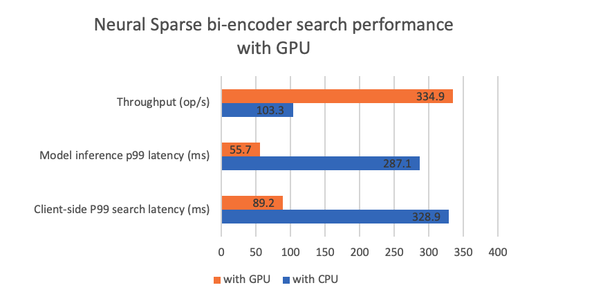
Using a GPU at search time

Our experiments show that using a GPU reduces the model inference latency by a large margin. This translates to significant improvements in the client-side search latency and throughput, as shown in the following figure. This performance boost is crucial for running neural sparse search in bi-encoder mode in production.

Using a GPU at ingestion time

Ingestion relies heavily on model inference, so using a GPU at ingestion time leads to a higher ingestion throughput. In our experiment, we used the same GPU endpoint for ingestion. We performed ingestion using 6 clients, with a bulk size of 10. The following figure illustrates the experiment results.

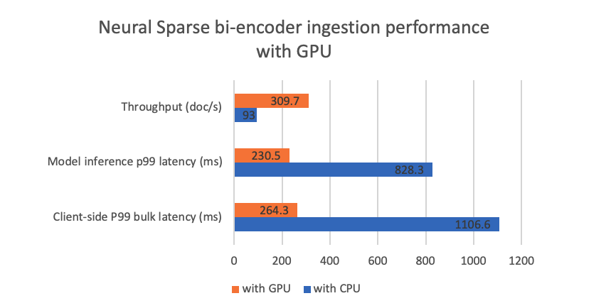
The GPU endpoint significantly accelerates the model ingestion process, achieving a
tripled throughput at a considerably lower cost. This is particularly valuable in scenarios with heavy ingestion workloads, regardless of whether you’re using the bi-encoder mode or the doc-only mode for search.

Conclusions

In this blog post, we explored the performance of neural sparse search and showed our experimental data. Here are some key takeaways:

1. Neural sparse search consists of tokenizer/model inference and inverted index search. The inverted index search latency grows linearly with the number of documents.
2. In our quantitative study on the MS MARCO dataset, the inverted index search workload in the doc-only mode is about 1.8x that of BM25, and in the bi-encoder mode, it is about 4x that of the doc-only mode.
3. OpenSearch 2.12 and later versions benefit from the performance improvements of the new Lucene version. These improvements accelerate both BM25 and neural sparse search on inverted indexes. Neural sparse search benefits more from this upgrade compared to BM25.
4. Model inference is a throughput bottleneck for neural sparse ingestion and bi-encoder search. Using a GPU can significantly accelerate model inference, leading to a higher throughput and better cost/performance ratio.

This study provides insights to help you scale your resources effectively when migrating from BM25 to neural sparse search in a new cluster. Refer to the quantitative data to estimate the workload requirements for your specific use case. If you require a high ingestion throughput or a high query throughput for searching in the bi-encoder mode, we recommend using a GPU. For more information about configuring neural sparse search, see the Neural sparse search documentation.